A Recurrent Neural Networks Primer - The Code
Recurrent Neural Networks - Code
After understanding the derivation from Mathematics of RNNs we can translate it into code. First, I’m going to use Python and numpy. You can find the code in a gist here.
RNN parameter definition
We start the code by defining the dimensions of the RNN we’re going to build:
# Configuration
## RNN definition
### maximum length of sequence
T = 6
### hidden state vector dimension
hidden_dim = 32
### output length
output_dim = 8
T is the length of the input sequence we’re going to use to predict the output. The way the RNN algorithm works, this is also the number of times we perform the inner loop of the RNN (the stuff in the \(\sigma\) function). Larger dimensions provide more information and make it easier to learn, but also create a problem due to vanishing gradients (which can be avoided using other algorithms like LSTM, GRU).
hidden_dim is the dimension of the hidden state. Larger dimensions make it easier to fit arbitrary functions, but also make it more difficult to optimize/train.
output_dim is the number of data points we want to predict. In many other implementations this is of dimension 1 (e.g. Karpathy’s char-rnn).
Training routine parameters
We use a simple stochastic gradient descent algorithm to train our neural net.
## training params
### cutoff for linear gradient
alpha = 0.025

### learning rate
eps = 1e-1
### number of training epochs
n_epochs = 10000
### number of samples to reserve for test
test_set_size = 4
### number of samples to generate
n_samples = 50
Most of these parameters are standard and I won’t go into them. However, the alpha parameter is important.
alpha is a length cutoff for the transition between \(L_2\) and \(L_1\) optimization objectives. For values of \(\|\Delta {y}\| \gt\) alpha The gradient is \(L_1\). Inside the alpha cutoff it is the softer \(L_2\) objective. This helps to prevent rapidly fluctuating gradients when the optimization converges close to \(\|\Delta {y}\| = 0\) but pushes parameters towards it. Later, when we plot some of the convergence plots you will see the instability when using the bare \(L_1\) objective.
Weight Matrix initialization
We initialize the weight matrices using some common matrix factorizations to make them more well behaved (and hopefully converge faster).
rng = np.random.default_rng(2882)
# the "hidden layer". aka the transition matrix. these are the weights in the RNN.
#    shape: hidden_dim x hidden_dim
W = rng.normal(0, (hidden_dim * hidden_dim) ** -0.75, size=(hidden_dim, hidden_dim))
_, W = np.linalg.qr(W, mode='complete')

# input matrix. translates from input vector to W
#     shape:  hidden_dim x T
U = rng.normal(0, (hidden_dim * T) ** -0.75, size=(hidden_dim, T))
svd_u, _, svd_vh = np.linalg.svd(U, full_matrices=False)
U = np.dot(svd_u, svd_vh)

# output matrix. translates from W to the output vector
#     shape:  output_dim x hidden_dim
V = rng.normal(0, (output_dim * hidden_dim) ** -0.75, size=(output_dim, hidden_dim))
svd_u, _, svd_vh = np.linalg.svd(V, full_matrices=False)
V = np.dot(svd_u, svd_vh)
The W matrix is square, so we can use a QR factorization to generate an upper triangular matrix for W. Being upper triangular is nice because they’re easier to solve using linear algebra. In an optimization process it just means that the columns are linearly independent. Linear independence allows each column of weights evolve independently as we descend the gradient.
Both the V and U matrices are not square. For those we choose a SVD decomposition. This creates an orthogonal matrix where the singular values all set to one. We multiply the svd_u and svd_vh terms back together to get the right shape for the weight matrix.
Formulas
# this is the formula used to update the hidden state
def new_hidden_state(x, s):
    u = np.dot(U, x)
    w = np.dot(W, s)
    rv = 1 / (1 + np.exp(-(u + w)))
    return rv

def el_mul(v, m):
    r = np.zeros_like(m)
    for c in range(r.shape[1]):
        r[:, c] = v * m[:, c]
    return r

def l_grad(dy):
    return np.array([np.maximum(np.minimum(1.0,y),-1.0) for y in dy])
You’ll recognize the new_hidden_state method as the sigmoid function. THis is used to compute the new hidden state from the old one, an input, and the weight matrices.
el_mul is an element wise multiplication method where you operate a row vector on the rows of a matrix.
l_grad is the loss objective we’re minimizing. If you wanted to experiment with other loss objectives, this is where you would plug in the gradient to see how they work. We’re using a version of the Huber loss function.
Training data setup
For this problem we’re going ot fit a sine function on a grid. We want to start form the number of training samples and test samples we want to generate and then use that to compute the right length sine wave. Each data point must consist of T + output_dim points (input plus output dimensions).
# set up training data:
#      let's use sin as out target method.
x_grid = np.linspace(0, 4 * np.pi, num=n_samples + test_set_size + T + output_dim)
dx_grid = x_grid[1] - x_grid[0]
sin_wave = np.sin(x_grid)
n_data_points = sin_wave.shape[0]
n_samples = n_data_points - T - output_dim
X = []
for i in range(0, n_samples):
    X.append(sin_wave[i : i + T + output_dim])

np.random.shuffle(X)
X_test = X[:test_set_size]
X = X[test_set_size:]
To generate the test data (which we plot below) we shuffle the training data and pick the first test_set_size samples.
Convenience methods
def plot_tests(step):
    v_lines = []
    for plot_i, x_y in enumerate(X_test):
        xs = x_y[:T]
        ys = x_y[T:]
        rnn_s = np.zeros(hidden_dim, dtype=np.float64)
        for t in range(T):
            x_i = np.zeros(T, dtype=np.float64)
            x_i[t] = xs[t]
            rnn_s = new_hidden_state(x_i, rnn_s)
        y_hat = np.dot(V, rnn_s)
        x = x_grid[:output_dim] + dx_grid*(output_dim + 1)*plot_i
        v_lines.append(dx_grid*(output_dim + 1)*plot_i - dx_grid)
        plt.plot(x, y_hat, "r")
        plt.plot(x, ys, "g")
    for x_pos in v_lines[1:]:
        plt.vlines(x_pos, -1, 1)
    frame1 = plt.gca()
    frame1.axes.get_xaxis().set_ticks([])
    frame1.set_ylim([-1.1,1.1])
    plt.savefig(f"step_plots/{step:06d}.png", format='png')
    plt.clf()
This method plots the test data in a single plot and writes it to an output directory. We can take these plots and convert them to a gif using ImageMagick: convert -delay 10 -loop 1 *.png gif_name.gif.
Algorithm
Here’s the full code block for the both computing the derivatives and predicting the output.
The prediction algorithm is actually pretty compact:
for x_y in X:
    xs = x_y[:T]
    ys = x_y[T:]
    rnn_s = np.zeros(hidden_dim, dtype=np.float64)
    for t in range(T):
        x_i = np.zeros(T, dtype=np.float64)
        x_i[t] = xs[t]
        rnn_s = new_hidden_state(x_i, rnn_s)
    dy = np.dot(V, rnn_s) - ys
First, we’re storing the sine wave in the X vector and have to split it up between the input and the output (xs and ys). Then we initialize our hidden state to the zero vector. For each data point we loop over all T input points. FOr each step, t, the x_i vector is initialized to zero except for the time step t we’re working on. We feed the old hidden state and the new x input to the new_hidden_state method and get back an updated hidden state. After working all the way through the input vector, we dot the V matrix into the hidden state and out pops the y prediction. Because this code is for both prediction and training we only store the error dy = \(\tilde{y} - y\) where np.dot(V, rnn_s) = \(\tilde{y}\).
Optimization
The bulk of the code is the optimization algorithm.
We start by scaling our learning rate by the number of samples. We want to average the gradient over all our training samples. It’s more efficient to just sum the gradients and scale the learning rate instead. For each pass over the training data (each epoch) we reset the cumulative variables.
eps = eps / n_samples
for e_i in range(n_epochs):
    loss = 0
    dL_dV = 0
    dL_dU = 0
    dL_dW = 0
Here’s the loop over training samples. Besides the things we need to do for evaluating the RNN on the new data, we are going to start accumulating the derivatives used in our stochastic gradient descent algorithm.
    for x_y in X:
        xs = x_y[:T]
        ys = x_y[T:]
        rnn_s = np.zeros(hidden_dim, dtype=np.float64)
        rnn_ds_dU = np.zeros((hidden_dim, T), dtype=np.float64)
        rnn_ds_dW = np.zeros((hidden_dim, hidden_dim), dtype=np.float64)
        for t in range(T):
            x_i = np.zeros(T, dtype=np.float64)
            x_i[t] = xs[t]
            p_rnn_s = rnn_s
            rnn_s = new_hidden_state(x_i, rnn_s)
rnn_ds_dU: This is \(\partial s / \partial \bar U\) for this sample. We will initialize it to zero and then accumulate it over T time steps.
rnn_ds_dW: This is \(\partial s / \partial \bar W\) for this sample. It’s accumulated the same as rnn_ds_dU.
p_rnn_s: We save the previous value of rnn_s for use in the rnn_ds_dW derivative.
            # derivs
            ds = rnn_s * (1 - rnn_s)
            ds_W = el_mul(ds, W)

            rnn_ds_dU = np.dot(ds_W, rnn_ds_dU)
            rnn_ds_dU += np.outer(ds, x_i)

            rnn_ds_dW = np.dot(ds_W, rnn_ds_dW)
            rnn_ds_dW += np.outer(ds, p_rnn_s)
You should be able to identify ds as the outer derivative of s=\(\sigma(x)\).
Both rnn_ds_dU and rnn_ds_dW include 2 terms, one is multiplying the current running total by the ds_W and the other is the product of either $s$ or $x$ and the current outer derivative. You can see this more clearly in the mathematical derivation.
One thing to note here is that this implementation has been optimized for computing the full derivative without truncation. We are able to loop over the time steps once (as opposed to the char-rnn implementation which makes a forward, then backward pass). If we wanted to truncate the backpropagation to a number of time steps, bptt_truncation_t, we could do so by altering this sum to start where t >= bptt_truncation_t.
        dy = np.dot(V, rnn_s) - ys

        rnn_dL_dV = np.outer(l_grad(dy), rnn_s)
        dyV = np.dot(l_grad(dy), V)

        loss_i = (0.5 * dy**2).sum()
        rnn_dL_dW = el_mul(dyV, rnn_ds_dW)
        rnn_dL_dU = el_mul(dyV, rnn_ds_dU)

        loss += loss_i
        dL_dV += rnn_dL_dV
        dL_dW += rnn_dL_dW
        dL_dU += rnn_dL_dU
Using l_grad we scale the loss gradient and accumulate the gradient over each sample.
    if (e_i + 1) % 100 == 0 or e_i == 0:
        print(
            f"{e_i}: total loss: {loss}\n\t\t<error> per data point: {np.sqrt(loss/n_samples/output_dim)}"
        )
        print(f"      dV range: {np.max(dL_dV) - np.min(dL_dV)}")
        print(f"      dU range: {np.max(dL_dU) - np.min(dL_dU)}")
        print(f"      dW range: {np.max(dL_dW) - np.min(dL_dW)}")
        plot_tests(e_i)
Every 100 steps we plot our current test set and print out loss and gradient magnitude information. We’re working to minimize hte loss objective over the sample set. In general, we expect the range of gradients to decrease as we improve the optimization. This isn’t true though, as sometime minimizing the overall loss might result in some weights having larger and other gradients smaller values. If these explode, we can tell something has gone wrong.
    W = W - eps * dL_dW
    V = V - eps * dL_dV
    U = U - eps * dL_dU
This is the step where we update the weights every epoch. Many more sophisticated methods are available to improve this simple update algorithm. For this problem, it’s good enough though.
Optimization
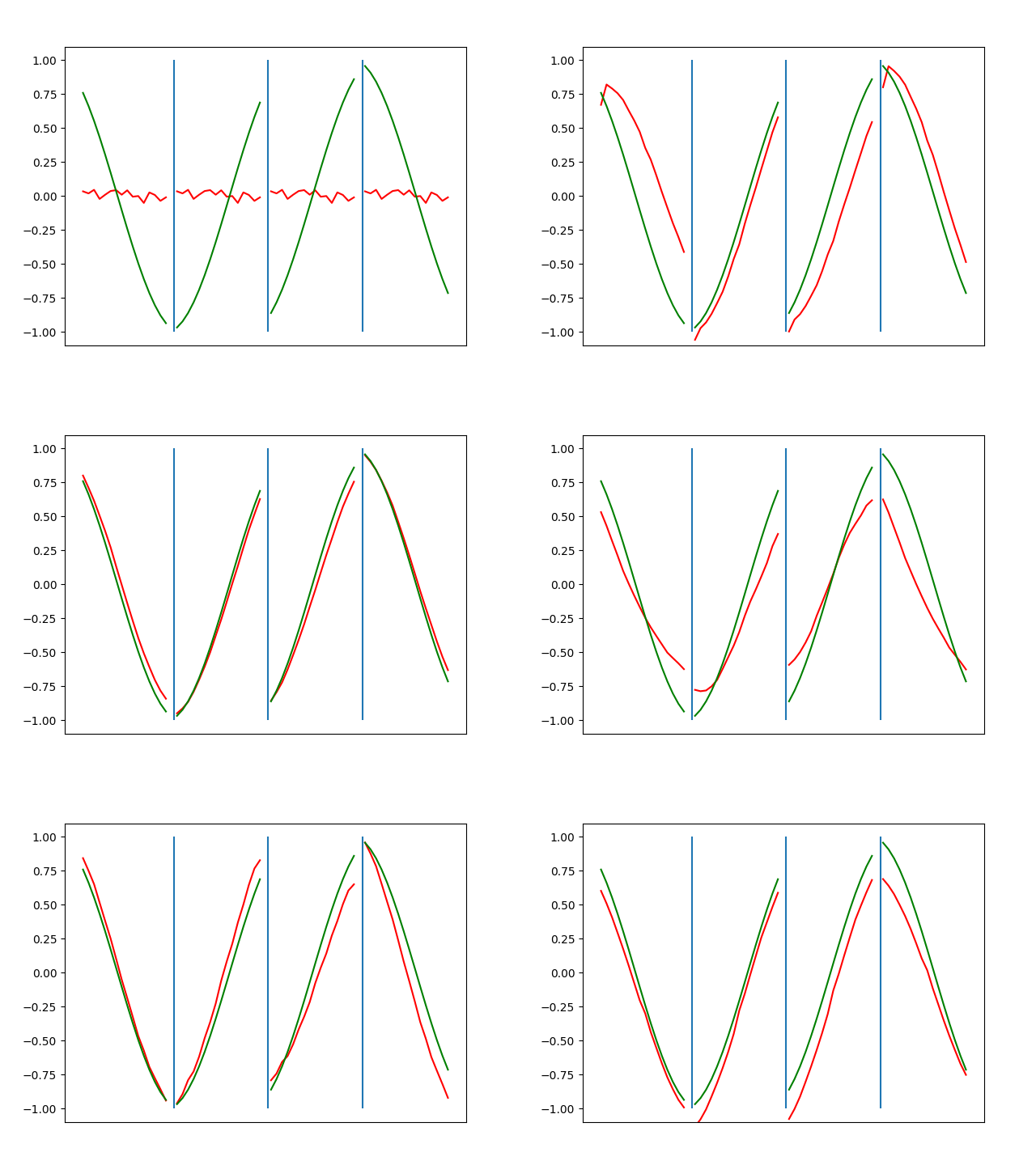
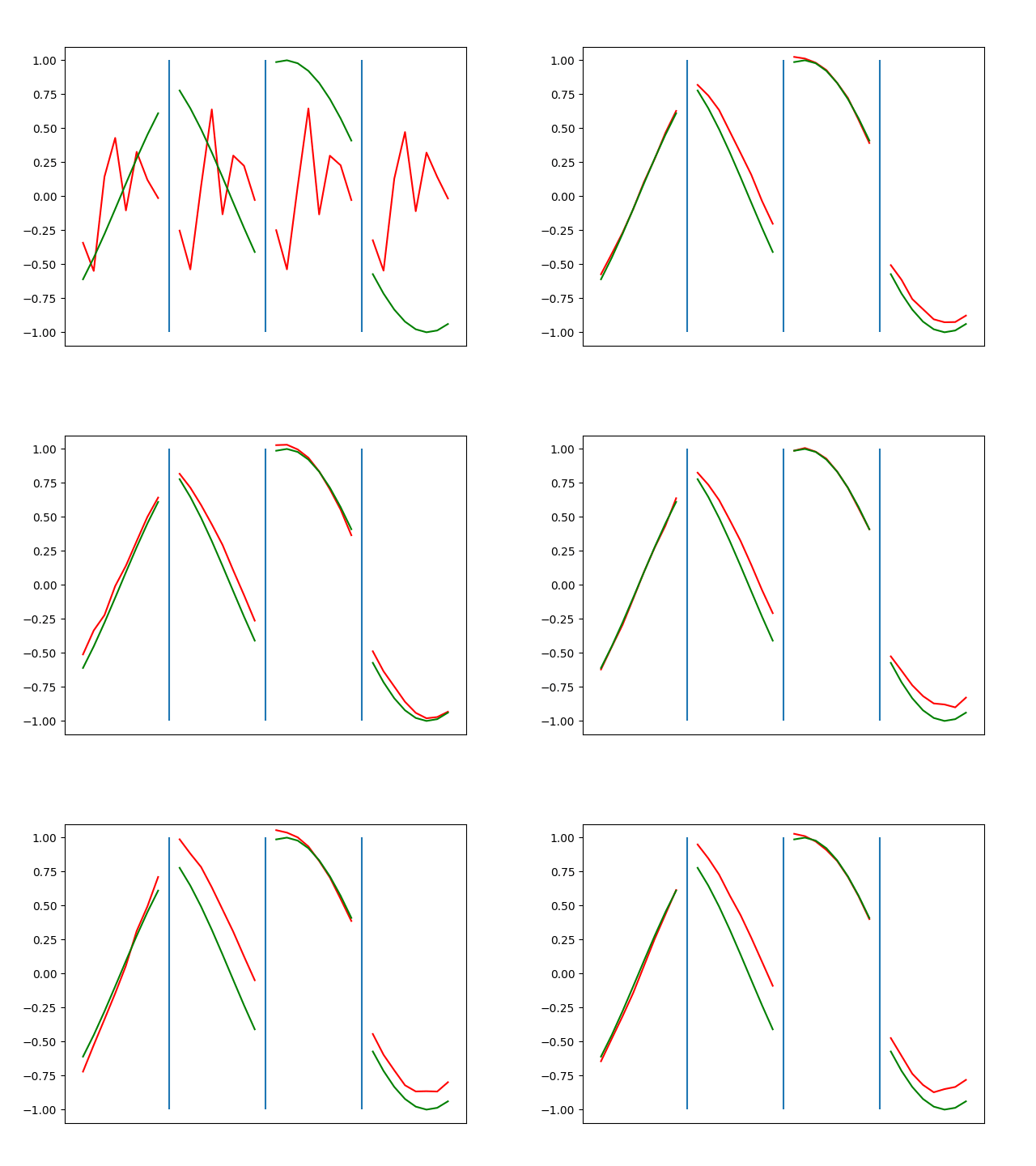
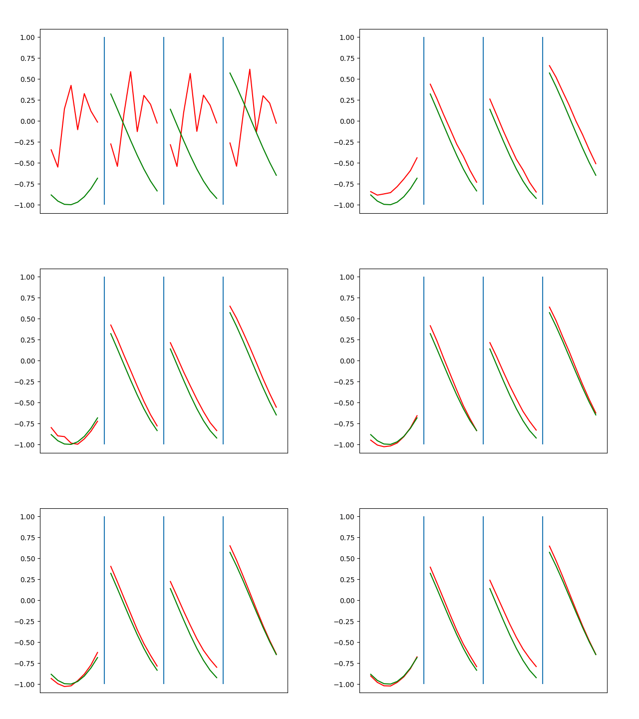
Below are plots depicting the RNN predictions converging from their random initial conditions to full optimization, and in some cases a little further. I randomly choose 4 segments to plot (that are not in the training set). The red line is our prediction $$\tilde y$ and the green line is the ground truth. This is the progress over 4000 epochs.

You can see it converges relatively quickly to the ground truth, but then starts to wiggle as you over optimize. I think that’s partly due to the cost function being pretty soft near $$\Delta y=0$. As mentioned earlier, we could choose any other loss function to optimize, or, to make things a little easier, simply change this gradient term.
For instance, if you want to use $L^1$ loss, you can change the term to:
\[\frac{\partial L_i}{\partial y_i} = \text{sgn}(\tilde{y}_j - y_j)\]where \(\text{sgn}\) is the sign function.
For elastic net:
\[\frac{\partial L_i}{\partial y_i} = \alpha[\text{sgn}(\tilde{y}_i - y_i)] + (1-\alpha)(\tilde{y}_i - y_i)\]Here’s a loss function that acts like $L^2$ near zero and $L^1$ away from it (soft near zero and not overly sensitive to outliers).
\[\begin{aligned} \frac{\partial L_i}{\partial y_i} &= \text{sgn}(\tilde{y}_i - y_i) \quad &\forall \quad |(\tilde{y}_i - y_i)| \geq \beta \\ &= (\tilde{y}_i - y_i) / \beta \quad &\forall \quad |(\tilde{y}_i - y_i)| \lt \beta \end{aligned}\]I spent some time tuning the optimization to be more stable. Here’s some elastic net action (if it is not looping, open in a new tab to see it evolve over epochs):

Ultimately I found the third loss function the best. It was pretty stable and worked fast.

Conclusion
The Recurrent Neural Network (RNN) remains a valuable tool for solving time series and natural language processing tasks. Understanding the algorithm and optimization techniques through detailed derivations and analysis can aid in developing a deeper intuition for RNNs. Please copy the code and run your own experiments!